Hebbian Learning through the lens of SAE traning.
Hebbian Learning through the lens of SAE traning.
- By Nikita Kurdiukov
- 2026-09-10 23:21:42Z
- 1 points
- Tag: Interpretability (ML & AI)
- Tag: Machine Learning (ML)
- Tag: Neuromorphic AI
- Tag: Sparse Autoencoders (SAEs)
- Tag: AI
- Personal Blog
- Comments: 0
- Post URL (HTML): /posts/7qjGWJcRSfMga46uR/hebbian-learning-through-the-lens-of-sae-traning
- Post URL (Markdown): /api/post/hebbian-learning-through-the-lens-of-sae-traning
- Comments URL (Markdown): /api/post/hebbian-learning-through-the-lens-of-sae-traning/comments
- Post URL (Markdown, compact): /api/post/hebbian-learning-through-the-lens-of-sae-traning?compact=1
Likely, modern competitive Hebbian learning rules train Sparse Autoencoders implicitly - and their approximations make them worse at it. These algorithms specify weight updates directly, without computing a loss and the consequent gradients. But their updates contain terms closely related to both. This raises a question: how much of their feature-learning behavior can we understand as approximate SAE optimization ?
This post develops that connection for tied-weight SAEs, identifies where the updates diverge, and presents a small experiment on language-model activations. For mechanistic interpretability, it might be interesting because Hebbian learning is connected to papers on Associative Memory that dig into its storage capacity.
The connection is concrete:
- Reconstruction terms in the loss ~ Hebbian terms
- Activation penalties ~ suppressive\negative (anti-Hebbian) terms
- Normalization supplies the projection correction
- Competition, coefficient choices, and omitted interactions determine how far a particular algorithm departs from exact tied-SAE descent
- Tying the weights makes updating one shared matrix update the whole SAE. There is no need for a second independently trained weight matrix. But both uses of that matrix still contribute to its derivative. This is why the comparison of a 2-layer SAE and 1 linear layer trained with some Hebbian learning rule1 is valid.
Below is the short argument and our small experiment on language-model activations. The full derivations, assumptions, and corrections to our paper are in the appendix.
This post hinges on a paper, initially published on NFAM workshop 2025. It was slightly updated in the new revision, whose Figures are posted here.
TLDR;
(0) Motivation. Selectivity of neurons to patterns in bio-inspired learning rules.
The authors of the work Unsupervised learning by competing hidden units, 2019 showcased that weights of a linear layer trained on CIFAR-10 using their biologically-inspired learning rule resemble input images (an image itself or an image prototype).
We conjectured that this neuronal selectivity is analogous to the feature selectivity exhibited by SAEs used for language model (LM) mechanistic interpretability research
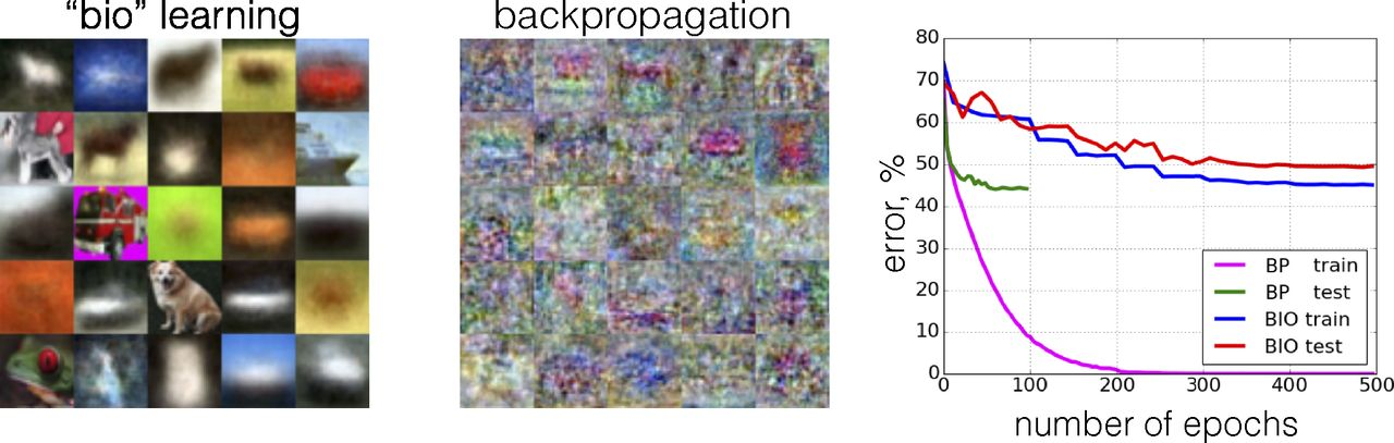
Fig. 7 from Unsupervised learning by competing hidden units, 2019.
"(Left) The weights learned by the network using the unsupervised learning algorithm. Twenty-five randomly chosen feature detectors of 2,000 are shown. (Center) The weights learned by the network trained end-to-end with the backpropagation algorithm. Twenty-five randomly chosen feature detectors of 2,000 are shown."
(1) The tip of the connection, in two equations.
Start with a linear, bias-free autoencoder whose encoder and decoder share weights:
Let . Its exact reconstruction anti-gradient is
The first term is the decoder contribution. Drop the second term, then discard the off-diagonal entries of , and each feature gets the familiar Oja update: .
That gives an explicit comparison: independent Oja updates omit the encoder contribution and cross-latent reconstruction interactions. This is algebra, not an analogy.
Sparsity adds another connection. For a unit-norm weight vector and positive activation :
- projected descent on an activation penalty moves along ;
- squared- descent moves along .
The latter is negative Oja. A tied ReLU SAE with one active latent, zero bias, and unit-norm weights even has the exact projected update : reconstruction attracts; the penalty repels.
Competitive SoftHebb (from ICLR 2023 paper) adds further choices. Its softmax coefficients and winner/loser signs differ from ordinary SAE gradients. These connections do not make its full update exact SAE descent. The appendix separates the identities from the approximations.
(2) Experiments. What happened on LM activations ?
We tested a SoftHebb-based encoder on 64-dimensional residual-stream activations from TinyStories-1M, using 3,200 ReLU latents. Each setup ran for five epochs under five seeds.
We compared:
- standard backpropagation (BP),
- tied-weight backpropagation (BP Tied),
- a Hebbian encoder with a trained decoder (BP Dec),
- a Hebbian encoder whose transposed weights decode (Hebb Tied).
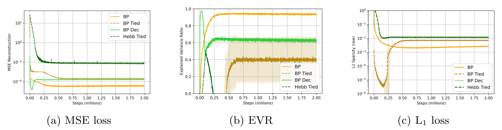
Paper Figure 1. Original training curves: reconstruction MSE, EVR, and L1 activation magnitude. Curves show mean ± standard deviation over five runs. The original EVR panel stops at zero, so it does not display the final negative Hebb Tied value.
Standard BP reached 0.929 EVR. The Hebbian encoder with a trained decoder reached 0.615; tied Hebbian decoding reached −0.520, worse than the mean-activation baseline under the reported metric. BP Tied reached 0.391 under the original initialization—but exceeded 0.90 after changing initialization. That change produced NaNs in the Hebbian setups.
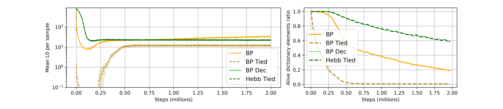
Paper Figure 2. Original sparsity curves: active latents per input and alive dictionary fraction. Hebbian setups overlap because they share encoder training. "Alive" concerns activity at evaluation, not cumulative activity since training began.
The Hebbian encoders activated about 22 latents per input, versus 32 for BP, while using roughly 59% of dictionary entries, versus 19% for BP. Broader dictionary usage does not itself establish better features. Here are selected activation patterns inspected on NeelNanda/pile-10k:
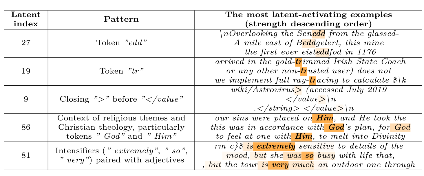
Paper Table 2. Examples of top samples and their contexts that activate latents in Hebbian tied weight SAE, Hebb Tied setup. The activating tokens are highlighted in orange, and the color opacity indicates activation strength.
(3) What to take from this.
The results fit the hypothesis worth testing: these Hebbian rules perform something related to SAE optimization, while departing from its exact updates. The experiment does not isolate which departure caused poor reconstruction. It also used training-subset reconstruction metrics, unmatched sparsity, nonzero encoder biases, and no explicit unit-norm constraint.
The next question is concrete: what happens if we restore the omitted update terms while controlling the other differences ? The derivation tells us what to change. The existing results motivate the test; they do not supply its answer.
(4) Prior work.
The broad link between Hebbian learning and sparse representations has a long history. Földiák (1990) studied sparse representations with local anti-Hebbian learning. Pehlevan and Chklovskii (2014) derived a local network from online nonnegative matrix factorization of input similarities; Hu, Pehlevan and Chklovskii (2015) derived online sparse dictionary learning from a regularized symmetric matrix-factorization objective. Plaut (2018) examined the relation between linear autoencoders and principal components. Our earlier ICLR 2025 workshop paper explored the LM application. This post contributes a worked comparison for the tied ReLU-plus- SAE, corrections to our published account, and a small empirical example.
Appendix. Derivations and paper corrections.
Read this appendix for an understanding the connection described.
If something like Appendix A.2.1 is referenced, it means the Appendix from this paper revision.
+++ A1. Start with the actual SAE loss.
Let be an input activation. Let contain feature vectors as rows. Write its -th row as , so is a column vector. Define
Weights are tied: the same detects features and reconstructs from them. Decoder bias is zero. No norm constraint yet.
The factor keeps derivatives clean. For the paper's convention , use and multiply the entire gradient below by two. This is an algebraic conversion; it does not assert identical optimizer dynamics under an arbitrary loss rescaling.
Write
Here is the reconstruction residual and records which ReLUs are active. Work away from ; at the kink, use the usual zero derivative convention.
The exact negative gradients are
Three pieces are visible in (3):
| Contribution to the update | Meaning |
|---|---|
| Change the decoding directions to reduce reconstruction error. | |
| Change which features the encoder activates to reduce that error. | |
| Reduce positive latent activations. |
Tying the weights makes these contributions add. Updating one shared matrix updates the whole SAE. There is no need for a second independently trained weight matrix. But both uses of that matrix still contribute to its derivative.
To see why, perturb by . With and fixed,
The reconstruction loss changes by . The sparsity loss changes by , because ReLU activations are nonnegative. Collect the coefficients of to obtain (3). Appendix A in the paper gives the same calculation one weight at a time.
+++
+++ A2. The reconstruction term already contains a Hebbian rule.
First take a linear encoder, , and set , . Equation (3) becomes
Expand just its decoder contribution:
This is the update expression in Oja's subspace algorithm, up to learning rate. The first term is Hebbian: output activity times input activity. The second subtracts the reconstruction contribution of the current features.
For feature , written as a column-vector update,
Now discard the cross-latent terms, equivalently replace by :
This is the single-neuron Oja rule, with .
Thus the general route from a tied linear AE gradient to independent Oja updates has two explicit omissions: the encoder contribution , and the off-diagonal terms in . Equation (6) is an exact identity; those omissions are approximations. Our paper’s Section 6 reverses the path attribution: it says the missing contribution is the decoder gradient. With the encoder/decoder conventions above, the subspace update retains the decoder-path contribution and omits the encoder-path contribution. This is a correction to the explanation, in addition to the duplicated term in Table 4.
Equation (6) also holds algebraically for ReLU outputs, but the full encoder term then has the gate . Calling an update "Oja's rule" additionally requires care about what its activity variable means.
A useful consequence: co-active latents interact in the reconstruction update. Independent Oja rules ignore those interactions. When at most one latent is active, the cross terms vanish exactly. Sparse activity reduces the number of possible interactions, but does not alone bound their total size.
+++
+++ A3. An exact special case: one active feature.
We can make the connection stronger without dropping a gradient term.
Assume zero bias, unit-norm rows, and exactly one active ReLU latent . Let
All other preactivations are strictly negative. Locally, the reconstruction is . Therefore
The active neuron's encoder reconstruction contribution vanishes. Inactive neurons have both and . The full reconstruction update is consequently
That is Oja's rule exactly, at this point in parameter space.
Now enforce the unit-norm constraint. Its tangent-space projector is
Since , projected descent on the full reconstruction-plus- loss gives
Here means the Euclidean gradient projected onto the unit sphere. The reconstruction term contributes ; the activation penalty contributes .
The sign now has a simple meaning:
- : move toward the input along the sphere.
- : move away, reducing the activation.
- : the two contributions cancel.
This is a precise setting in which a tied SAE produces Hebbian and anti-Hebbian behavior from the same loss. The sign depends on activation magnitude relative to ; it is not the same rule as assigning a positive update to the winner and negative updates to every loser.
All three special-case assumptions need qualification in the experiment. The Hebbian setups averaged about 22 active latents per input; Appendix A.2 reports no explicit decoder-weight normalization; and Appendix A.2.1 sets bias = True. Exact unit norm and zero encoder bias were therefore not enforced. Equation (10) is an explanatory special case, not an exact description of those runs.
+++
+++ A4. Why negative updates resemble activation penalties.
The unit sphere also makes the penalty connection easy to derive on its own. Take one weight vector , no bias, , and . Then (recall )
For any differentiable scalar penalty (just some function for now, do not startle), the chain rule gives
For positive activation :
| Penalty | Projected negative gradient | ||
|---|---|---|---|
| $ lambda |
u |
$ | |
The first is a constant-strength repulsive direction. The second is negative Oja, with repulsion weighted by the activation.
For an unconstrained weight vector, the respective negative gradients are just and on the positive branch. The correction comes from projection/normalization. It is not present in the ordinary unconstrained sparsity gradient.
Two distinctions matter. For signed linear activations, the coefficient is . For , both penalties have zero gradient on the inactive branch . Also, squared suppresses activation magnitude; it does not have the same zero-inducing behavior as .
The direction really does suppress a positive response. Under a continuous update
This concerns response to the current input. It does not prove mutual orthogonality of learned features or recovery of independent concepts.
The geometry requires unit norm, which is favorable in the SAE as well2. In general,
Away from the sphere, the Oja direction includes a radial component. A finite Euler step also leaves the sphere by a second-order amount, so exact constrained optimization requires renormalization or another suitable constrained update. Unit-norm rows do not mean orthogonal rows; a 3,200-row dictionary in 64 dimensions cannot have all rows mutually orthogonal.
+++
+++ A5. Where the competitive SoftHebb rule fits.
Separate three quantities that are easy to mix:
Here is the raw score (preactivation), the SAE code (activation), and a softmax competition weight (where the method name comes from). For this comparison, biases are omitted. Notation clarification: Table 4 writes inside its softmax and normalization term. That symbol must not silently inherit the post-ReLU meaning from the SAE definition. Equation (13) below uses the preactivation explicitly; the implementation qualification follows the equation. A bias-free competitive variant has the form
The checked upstream implementation computes competition from preactivations. HebbSoftKrotovLinear defaults to mode = 0, with positive winner and negative losers; it also has rank-selected modes. Bias enters the preactivation when enabled. Updates are batch-aggregated and rescaled, with additional bias and learning-rate machinery. The coefficient is exact for mode 0. The schematic simplifications in (13) are omitted bias, batch aggregation, update rescaling, and learning-rate machinery.
Appendix A.2.1 reports t_invert = 50. The upstream activation function uses , equivalent to . That does not establish near-hard competition without the score gaps. If is the largest score,
With 3,200 equal scores, at any positive temperature. With well-separated scores it can approach one. Winner-probability or entropy measurements would establish which regime the runs occupied.
On unit-norm rows (recall ), (13) is . Its geometry matches the attraction/repulsion directions above. Its coefficient generally differs:
- Oja uses .
- Projected descent on an active latent uses a constant negative coefficient.
- Projected squared- descent uses a coefficient proportional to .
- The competitive rule uses , which depends on every score and on winner selection.
For a loser with , can be read as projected descent with an input-dependent step size, or as projected squared- descent with step size . This is a pointwise direction match. It does not identify the rule with ordinary descent on one fixed weighted SAE loss. For an inactive ReLU latent, that direction match fails: its SAE penalty gradient is zero, whereas its competitive update can be nonzero.
One further subtlety: writing as a proposed loss does not solve the problem. Differentiating it also differentiates . Freezing those weights during differentiation defines a surrogate update, not the ordinary gradient of that expression.
The distinction between magnitude and rank (i.e. top-1, top-2 neuron, etc) is worth discussing. Equation (10) changes sign at an activation threshold. Equation (13) changes sign according to who wins. The rank-selected Krotov variant tabulated in Table 4 uses a constant negative coefficient on the selected neuron, matching projected descent on a positive activation up to that coefficient. This is a comparison to the tabulated rule, not a claim about which experimental mode ran.
The upstream rank modes differ. Mode 1 assigns the selected neuron coefficient ; mode 2 assigns . Other neurons retain in both modes. Only mode 2 has a constant selected-neuron coefficient. Even there, the full update norm need not be constant: it also depends on .
The useful connection is explicit: reconstruction supplies Hebbian terms; activation penalties supply suppressive (anti-Hebbian) terms; normalization supplies the projection correction. Competition, coefficient choices, and omitted interactions determine how far a particular algorithm departs from exact tied-SAE descent.
+++
+++ A6. (Optional) Coordinate derivation.
Use for an input coordinate, for a latent, and for a reconstructed coordinate. From (1),
The first term differentiates the decoder use of ; the second differentiates the encoder use. Hence
Because for ReLU,
Combining them reproduces (3). This also fixes the transpose/shape conventions: each term is .
For a general elementwise activation and a differentiable penalty , the same argument yields
For linear signed codes with , use and away from zero. For a batch-mean loss, average the per-input gradients. Additional coordinate-wise normalizations of MSE or sparsity must be included explicitly in the coefficients.
The exact per-row ReLU update is another useful way to inspect the omissions:
This is a direct algorithm for updating the shared SAE matrix. An autodiff engine is optional. The residual and cross-feature sums remain required for exact descent; removing autodiff does not make those dependencies disappear. "Local" therefore needs a specified meaning: layer-local computation is different from a rule using only one synapse's weight and its pre/post activities.
+++
+++ A7. (Optional) Does the signed-softmax field have a scalar potential ?
Even with winner identity fixed, the score-space coefficient field is generally not the Euclidean gradient of a scalar potential. For ,
These cross derivatives differ when . A smooth scalar potential would require them to agree. This rules out that particular ordinary score-space gradient interpretation. It does not rule out a metric-dependent optimization view, a surrogate construction, a Lyapunov function, or an interpretation with additional state.
+++
+++ A8. Experimental table from the paper.
Mean standard deviation over five runs, transcribed from Table 1 in the paper. Metrics use the training subset. Dictionary counts reflect the paper's reported activity metric; the precise evaluation window requires its implementation.
| Setup | Explained variance ratio (EVR) | Active latents per input | Reported dictionary size |
|---|---|---|---|
| Backpropagation encoder and decoder | 0.929 ± 0.012 | 32.4 ± 2.08 | 612 ± 17.5 |
| Backpropagation, tied weights | 0.391 ± 0.271 | 12.0 ± 2.40 | 24.2 ± 5.7 |
| Hebbian encoder, trained separate decoder | 0.615 ± 0.025 | 22.3 ± 1.96 | 1,890 ± 53.8 |
| Hebbian encoder, tied decoder | −0.520 ± 0.110 | 22.3 ± 1.96 | 1,890 ± 53.8 |
+++
+++ A9. Corrections to the paper.
- Table 4 labels its fast-AI Krotov implementation with the 2018 citation; the competitive-hidden-units work is actually the 2019 paper named "Unsupervised learning by competing hidden units".
- The special-case (see A3. An exact special case: one active feature.) derivation here is an explanatory extension; it is not a new experiment or a claim of historical priority.
- Correction to the paper's Table 4:
- its two bracketed terms for the linear tied AE both simplify to . The full negative gradient is , as in (5). The subspace term is the decoder-path contribution under the conventions used here.
- Section 6 also names the omitted path incorrectly: it is the encoder contribution, not the decoder contribution.
- Separately, Equation (13) (from A5. Where the competitive SoftHebb rule fits.) makes the preactivation/SAE-code notation explicit rather than carrying over Table 4’s ambiguous .
- These corrections above concern the derivation and its interpretation; they do not by themselves establish an error in the experimental implementation.
+++
Which can contain a non-linear activation, like in the SoftHebb methods.↩
Almost every major library (including SAELens) strictly enforces a unit norm constraint on the decoder weights. After every optimizer gradient step, libraries explicitly normalize the dictionary vectors or use a projection step to clamp the column norms of the decoder matrix back to exactly 1.↩